Morris Screening Method
Screening methods are used to rank the importance of the model parameters using a relatively small number of model executions [1]. However, they tend to simply give qualitative measures. That is, meaningful information resides in the rank itself but not in the exact importance of the parameters with respect to the output. These methods are particularly valuable in the early phase of a SA to identify the non-influential parameters of a model, which then could be safely excluded from further detailed analysis. This exclusion step is important to reduce the size of the problem especially if a more expensive method is to be applied at the next step. In this work, attention was paid to a particular screening method proposed by Morris [2].
Elementary Effects
Consider a model with \(K\) parameters, where \(\vec{x} = (x_1, x_2, . . ., x_K)\) is a vector of parameter value mapped onto the unit hypercube and \(y(\vec{x})\) is the model output evaluated at point \(\vec{x}\). The elementary effect of parameter k is defined as follow [2] ,
\(EE_k = \frac{Y(x_1, x_2, \ldots, x_k + \Delta, \ldots, x_K) - Y(x_1, x_2, \ldots, x_K)}{\Delta}\)
Where \(\Delta\), the grid jump, is chosen such that \(\vec{x} + \Delta\) is still in the specified domain of parameter space; \(\Delta\) is a value in \({\frac{1}{p-1}, \ldots, 1 - \frac{1}{p-1}}\) where \(p\) is the number of levels that partitions the model parameter space into a uniform grid of points at which the model can be evaluated. The grid constructs a finite distribution of size \(p^{K-1} [p - \Delta(p-1)]\) elementary effects per input parameters.
The key idea of the original Morris method is in initiating the model evaluations from various “nominal” points \(\vec{x}\) randomly selected over the grid and then gradually advancing one grid jump at a time between each model evaluation (one at a time), along a different dimension of the parameter space selected randomly.
Statistics of Elementary Effects and Sensitivity Measure
Consider now that an \(n_R\) number of elementary effects (or replicates) associated with the k’th parameter have been sampled from the finite distribution of \(EE_k\). The statistical summary of \(EE_k\) from the sampled trajectories can be calculated. The first is the arithmetic mean defined as,
\(\mu_k = \frac{1}{n_R} \Sigma^{n_R}_{r=1} EE^{r}_{k}\)
The second statistical summary of interest is the standard deviation of the elementary effect associated with the k’th parameter from all the trajectories,
\(\sigma_k = \sqrt{\frac{1}{n_R}\Sigma^{n_R}_{r=1} (EE^{r}_{k} - \mu_k)^2}\)
The standard deviation gives an indication of the presence of nonlinearity and/or interactions between the k’th parameter and other parameters. As a change in a parameter value might have a changing sign on the output and thus result in a cancelation effect (as can be the case for a nonmonotonic function), Campolongo et al. [4] proposed the use of the mean of the absolute elementary effect to circumvent this issue. It is defined as
\(\mu^{*}_k = \frac{1}{n_R} \Sigma^{n_R}_{r=1} |EE^{r}_{k}|\)
The three aforementioned statistical summaries, when evaluated over a large number of trajectories \(n_R\), can provide global sensitivity measures of the importance of the k’th parameter. As indicated by Morris [2] there are three possible categories of parameter importance:
- Parameters with noninfluential effects, i.e., the parameters that have relatively small values of both \(\mu_k\) (or \(\mu^{*}_k\)) and \(\sigma_k\). The small values of both indicate that the parameter has a negligible overall effect on the model output.
- Parameters with linear and/or additive effects, i.e., the parameters that have a relatively large value of \(\mu_k\) (or \(\mu^{*}_k\)) and relatively small value of \(\sigma_k\). The small value of \(\sigma_k\) and the large value of \(\mu_k\) (or \(\mu^{*}_k\)) indicate that the variation of elementary effects is small while the magnitude of the effect itself is consistently large for the perturbations in the parameter space.
- Parameters with nonlinear and/or interaction effects, i.e., the parameters that have a relatively small value of \(\mu_k\) (or \(\mu^{*}_k\)) and a relatively large value of \(\sigma_k\). Opposite to the previous case, a small value of \(\mu_k\) (or \(\mu^{*}_k\)) indicates that the aggregate effect of perturbations is seemingly small while a large value of \(\sigma_k\) indicates that the variation of the effect is large; the effect can be large or negligibly small depending on the other values of parameters at which the model is evaluated. Such large variation is a symptom of nonlinear effects and/or parameter interaction.
Such classification makes parameter importance ranking and, in turn, screening of non-influential parameters possible. However, the procedure is done rather qualitatively, and this is illustrated in the figure below, which depicts a typical parameter classification derived from visual inspection of the elementary effect statistics on the \(\sigma_k\) versus \(\mu^{*}_k\) plane.

The notions of influential and non-influential parameters are based on the relative locations of those statistics in the plane. Typically, the non-influential ones are clustered closer to the origin (relative to the more influential ones) with a pronounced boundary such as depicted in the figure. Admittedly, if these statistics are spread uniformly across the plane, the distinction would be more ambiguous (in this case, a more advanced classification such as the ones based on clustering techniques might be helpful). Furthermore, for a parameter with large \(\mu_k\) and \(\sigma_k\), the method cannot distinguish between non-linearity effects from parameter interactions on the output.
Design of Experiment for Screening Analysis
There are two available experimental designs for to carry out the Morris
screening method in gsa-module: the trajectory design and radial OAT
design.
Trajectory Design (Winding Stairs)
Trajectory design is the original Morris implementation of the design of experiment for screening design [2]. Essentially, it is a randomized one-at-a-time design where each parameter is perturbed once, similar to that of the winding stairs design proposed by Jansen et al. [3]. The most important feature of trajectory design is that it does not return to the original base point after perturbation, but continue perturbing another dimension for the last perturbed point. This ensures more efficient parameter space exploration although requires additional user-defined parameter called level [4].
A trajectory design is defined by the number of trajectories (r), the number of levels (p), and the number of model parameters (k). Each trajectories evaluate the model (k + 1) times so the economy of it in computing the elementary effects statistics is r * (k+1) code runs.
A randomized trajectory design matrix is given by \(b^*\) ([2], [5]),
- \(b\): a strictly lower triangular matrix of 1s, with dimension of (k + 1)-by-k
- \(x^*\): Random starting point in the parameter space, with dimension of (k + 1)-by-k - each row is the same.
- \(d^*\): a k-dimensional diagonal matrix which each element is either +1 or -1 with equal probability. This matrix determines whether a parameter value will decrease or increase.
- \(p^*\): k-by-k random permutation matrix in which each row contains one element equal to 1, all others are 0, and no two columns have 1s in the same position. This matrix determines the order in which parameters are perturbed.
- \(j_k\): (k + 1)-by-k matrix of 1s
- \(\Delta\): factorial increment in a diagonal matrix of (k + 1)-by-(k + 1)
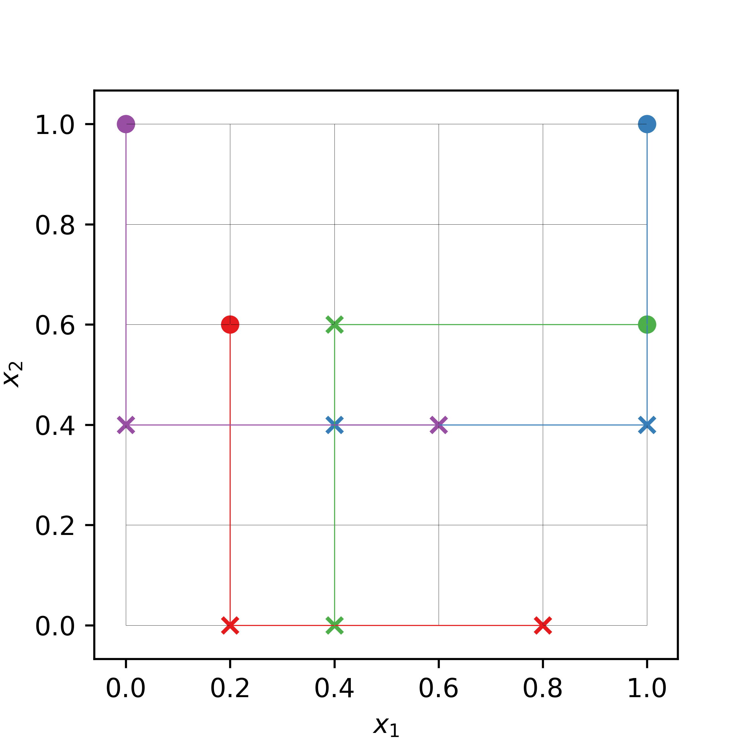
The following is an example of a trajectory design in 2-dimensional input space with 4 trajectories (or replicates). The input parameter space is uniformly divided into 6 levels. The filled circles are the random base (nominal) points from which the random perturbation of the same size (i.e., the grid jump) is carried out one-at-a-time.
Radial Design
Radial design is a design for screening analysis proposed in [4]. Similar to trajectory design it is based on an extension of one-at-a-time design. In the implementation of [4], Sobol’ quasi-random sequence is used as the basis. Its main advantage over the trajectory design is that the specification of input discretization level by user is no longer required. Furthermore, the grid jump will also be varying from one input dimension to another, and from replicate to replicate incorporating additional possible sources of variation in the method.
- The procedure to generate radial design of r replicates is as follow:
- Generate Sobol’ sequence with dimension (r+R, 2*k). R is the shift to avoid repetition in the sequence. The value of R is recommended to be fixed at 4 following [4], but see Choosing Shifting Value below for additional comments.
- The first half of the matrix up to the r-th row will serve as the base points: \(a_i = (x_{i,1}, x_{i,2}, \ldots x_{i,k}) \; ; i = 1,\ldots r\). The second half of the matrix, starting from the R+1-th row will serve as the auxiliary points, from which the perturbed states of the base point are created: \(b_i = (x_{R+i,k+1}, x_{R+i,k+2}, \ldots x_{R+i,2k}) \; ; i = 1,\ldots r\)
- For each row of the base points, create a set of perturbed states by substituting the value at each dimension by the value from the auxiliary points at the same dimension, one at a time. For each base point, there will be additional k perturbed points. For instance the 1st perturbed point of the i-th base point a_i is \(a^{*,1}_i = (x_{R+i,k+1}, x_{i,2}, \ldots x_{i,k})\), while the second is \(a^{*,2}_i = (x_{i,1}, x_{R+i,k+2}, \ldots x_{i,k})\). In general the j-th perturbed point of the i-th base point is \(a^{*,j}_i = (x_{i,1}, \ldots x_{R+i,k+j}, \ldots x_{i,k})\).
- A single elementary effect for each input dimension can be computed on the basis of function evaluations at k+1 points: 1 base point and k perturbed points.
- Repeat the process until the requested r replications have been constructed.
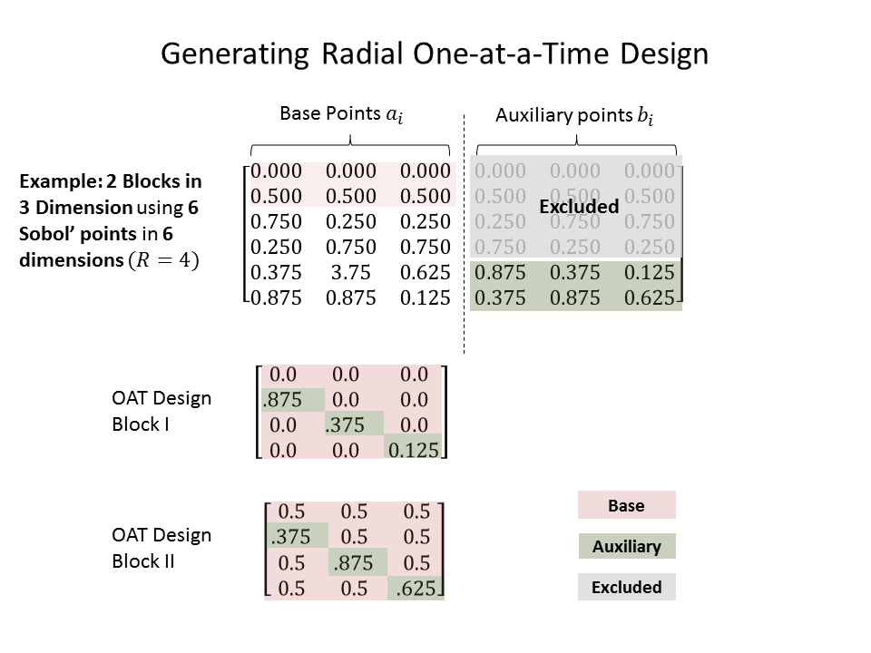
An illustration of radial OAT design generation based on Sobol’ sequence can be seen in the figure below.
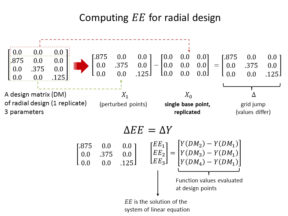
As such the radial design has the same economy as the trajectory design, that is r * (k+1) computations for a k-dimensional model with r replications. The computation of the elementary effect \(EE_i\), however, is slightly different due to the fact that now the grid jump differs for each input dimension at each replication.
- \(y(a^{*,j}_i)\): function value at j-th perturbed point of the i-th replicate.
- \(y(a_i)\): function value at the base point of the i-th replicate.
- \(x_{R+i,k+j}\): the perturbed input at dimension j of the i-th replicate.
- \(x_{i,j}\): the base input at dimension j of the i-th replicate.
As can be seen the average over many replications of the elementary effect defined above will automatically yield \(\mu^*\).
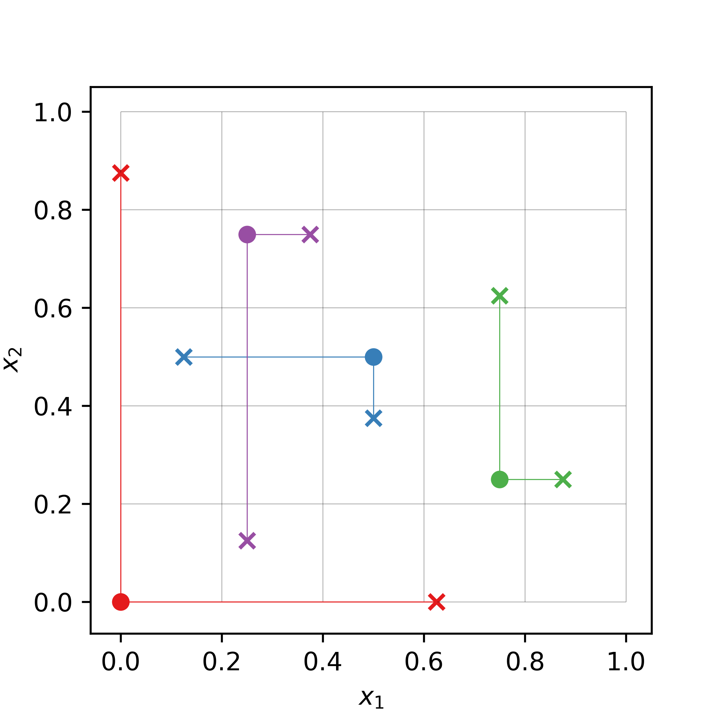
The following is an example of a radial design in 2-dimensional input space with 4 base points (filled circles), located not necessarily in a specific grid. The perturbations are carried out from these base points (crosses). The size of the perturbation differs from input dimension to input dimension and from replicate to replicate.
Choosing Shifting Value
As mentioned the recommendation given by [4] for the value of R is 4. This value reflects the fact that the a sample of Sobol’ sequence across dimension tends to repeat values, especially in the first several rows. For example, the first two Sobol’ samples used here have the values of 0.0 and 0.5 in all of the dimensions. If such repetition in value happened one or more rows in the \(\Delta\) matrix will be zero (so is the \(\Delta Y\) vector), and cause the system of linear equation to be under-determined.
But except for the obvious repetitions of values in different dimensions in the first several samples any other repetitions cannot be excluded to reoccur down the line of samples. As such the value of R has to be picked carefully and from our experience this value is highly dependent on the number of samples and/or dimension. Yet, the of the main points of using radial design in the first place was to avoid specifying the number of levels p. Choosing R for different number of samples and/or dimensions definitely defeat the purpose of using radial design.
A pragmatic solution for this problem, which is adopted here, is to check whether a given auxiliary point has the same value with the base point in one or more dimension, every time a block of one-at-a-time design is generated. If it has then use the next auxiliary point instead. Finally, to replace the missing auxiliary point, an additional point is generated using the Sobol’ sequence.
Miscellaneous Topics
Computation of the Elementary Effect
In gsa-module, computing the elementary effect for each replications is
achieved by using matrix algebra, which is similar to the implementation in
[6]. There is slight difference between the computation of elementary effects
for trajectory design and radial design.
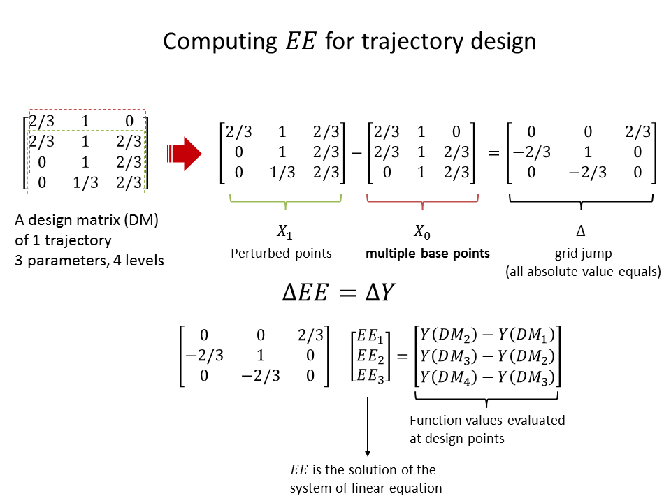
The following figure illustrate the computation of all the elementary effects
of a single replicate for 3-parameter model using trajectory design with
4 levels.
The following figure illustrate the same computation of a single replicate for 3-parameter model using radial design (no number of levels specification needed).
The statistics of the elementary effects are eventually computed after the same procedure are repeated for many replications.
Presenting the Results of the Analysis
Standardized Elementary Effect
In the original implementation of Morris method [2], the input parameter is normalized, that is all the parameters values lie between 0, 1. Furthermore, following the suggestion by Saltelli et al. [5], the grid jump size is kept constant for a given number of levels for all parameters. As such, the method is prone to misrank the important parameters if there is a vast difference in the original scale of various parameters (e.g., [0,1] in one parameter, [10,100] in another, etc.). The normalized scale of [0,1] would then be biased to the parameter who has the largest scale of variation. To compare the elementary effect in a common ground taking into account the original scale of variation for each parameter, it is advised in [7] to scale the elementary effect with the standard deviation of the input \(\sigma_{x_i}\) and of the output \(\sigma_y\),
In gsa-module, the standardized elementary effect is automatically computed
if the rescaled input parameters values are specified. It is used to compute
the standard deviation for each of the parameters taking into account the
original scale of variation of each.
Optimized Trajectory Design
References
| [1] | A. Saltelli et al., “Sensitivity Analysis in Practice: A Guide to Assessing Scientific Models,” John Wiley & Sons, Ltd. United Kingdom (2004). |
| [2] | (1, 2, 3, 4, 5, 6) Max D. Morris, “Factorial Sampling Plans for Preliminary Computational Experiments”, Technometrics, Vol. 33, No. 2, pp. 161-174, 1991. |
| [3] | Michiel J.W. Jansen, Walter A.H. Rossing, and Richard A. Daamen, “Monte Carlo Estimation of Uncertainty Contributions from Several Independent Multivariate Sources,” in Predictability and Nonlinear Modelling in Natural Sciences and Economics, Dordrecht, Germany, Kluwer Publishing, 1994, pp. 334 - 343. |
| [4] | (1, 2, 3, 4, 5, 6) F. Campolongo, A. Saltelli, and J. Cariboni, “From Screening to Quantitative Sensitivity Analysis. A Unified Approach,” Computer Physics Communications, Vol. 192, pp. 978 - 988, 2011. |
| [5] | (1, 2) A. Saltelli et al., “Global Sensitivity Analysis. The Primer,” West Sussex, John Wiley & Sons, 2008, pp. 114 |
| [6] | Jon D. Herman, SALib [Source Code], March 2014, https://github.com/jdherman/SALib |
| [7] | G. Sin and K. V. Gernaey, “Improving the Morris Method for Sensitivity Analysis by Scaling the Elementary Effects,” in Proc. 19th European Symposium on Computer Aided Process Engineering, 2009 |