Ishigami Function

Ishigami function is a 3-dimensional function introduced by Ishigami and Homma [1],

\[f(\mathbf{x}) = \sin x_1 + a \sin^2 x_2 + b x^4_3 \sin x_1\]

\[x_d \sim U[-\pi, \pi]; d = 1, 2, 3\]

the parameters a and b can be adjusted but have default values of 7 and 0.1, respectively.

Analytical Solution

The analytical formulas for the variance terms of the Ishigami function for \(\mathbf{X}_d \sim \mathcal{U}[-\pi,\pi]; \, d = 1, 2, 3\) and the given parameter \(a\) and \(b\) are the following

Marginal Variance

\[\mathbb{V}[Y] = \frac{a^2}{8} + \frac{b \pi^4}{5} + \frac{b^2 \pi^8}{18} + \frac{1}{2}\]

Top Marginal Variance

\[\begin{split}V_1 & = \mathbb{V}_{1} [\mathbb{E}_{2,3} [Y | X_1]] & = \frac{1}{2} \left(1 + \frac{b \pi^4}{5}\right)^2 \\ V_2 & = \mathbb{V}_{2} [\mathbb{E}_{1,3} [Y | X_2]] & = \frac{a^2}{8} \\ V_3 & = \mathbb{V}_{3} [\mathbb{E}_{1,2} [Y | X_3]] & = 0\end{split}\]

Bottom Marginal Variance

\[\begin{split}VT_1 = \mathbb{E}_{2,3} [\mathbb{V}_{1} [Y | \mathbf{X}_2,\mathbf{X}_3]] & = \frac{1}{2} \left(1 + \frac{b \pi^4}{5}\right)^2 + \frac{8 b^2 \pi^8}{225}\\ VT_2 = \mathbb{E}_{1,3} [\mathbb{V}_{2} [Y | \mathbf{X}_1,\mathbf{X}_3]] & = \frac{a^2}{8} \\ VT_3 = \mathbb{E}_{1,2} [\mathbb{V}_{3} [Y | \mathbf{X}_1,\mathbf{X}_2]] & = \frac{8 b^2 \pi^8}{225}\end{split}\]

The analytical main- and total-effect sensitivity indices can be computed using their respective definition in relation to the variance terms given above.

Morris Screening Results

The function was used to test the implementation of the Morris screening and most precisely that of the two designs of experiment: the trajectory and radial designs (see Morris Screening Method).

Trajectory sampling design

The trajectory effect is the original design proposed by Morris. The design matrix was generated with:

• number of trajectories (r) equal to 10, 100 and 1000 times the number of parameter (k=3),
• and levels (p) equal to 4, 8, 12 and 20.

Each generated design was used to evaluate the Morris modified function and the associated elementary effects were calculated.

The following figures show the \(\sigma\) vs. \(\mu^*\) plot for the four parameters of the Ishigami function for different sets of r and p values. Each set of (r, p) value was repeated 1000 times and a histogram of the results is presented for each parameter in the figures.

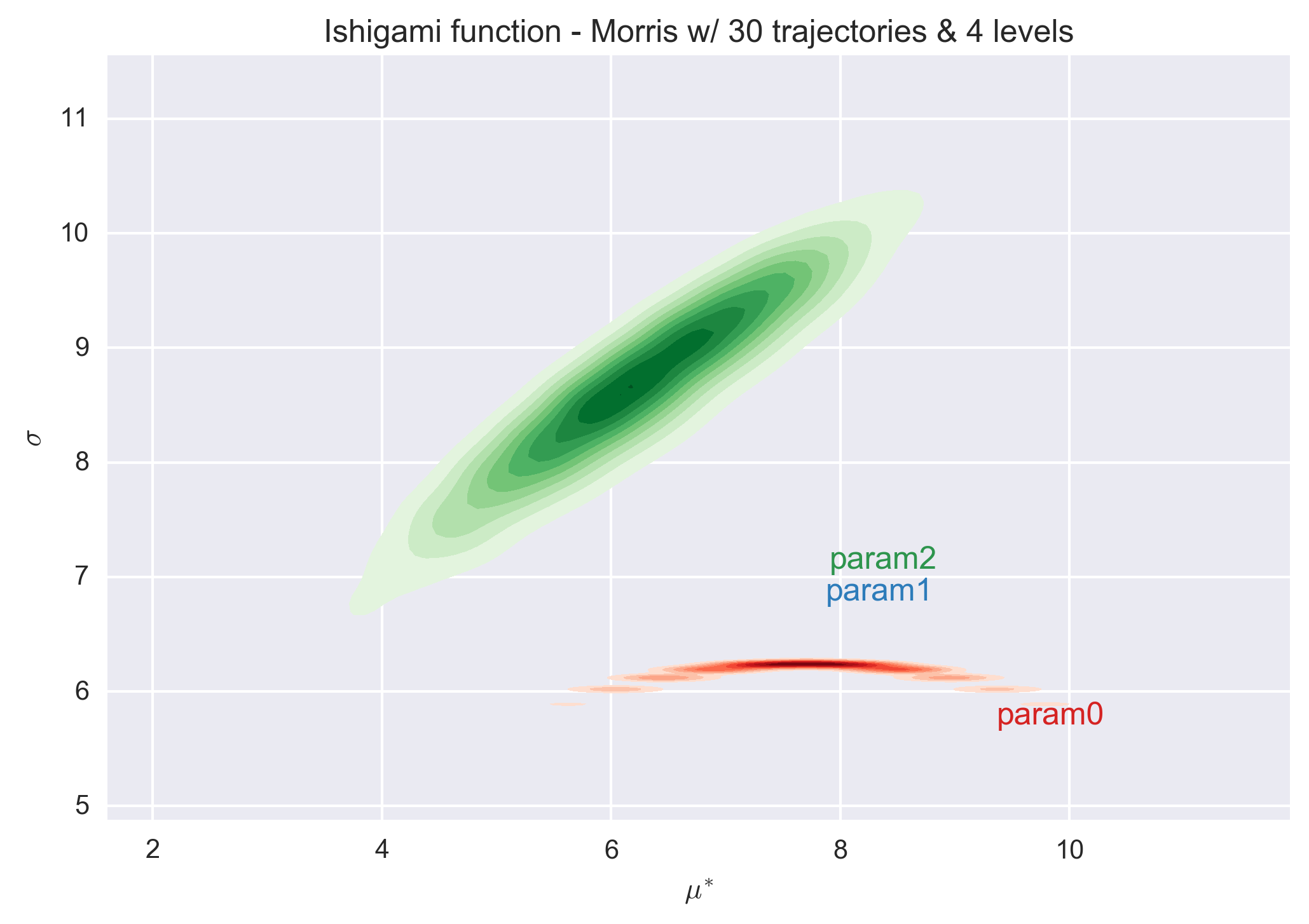
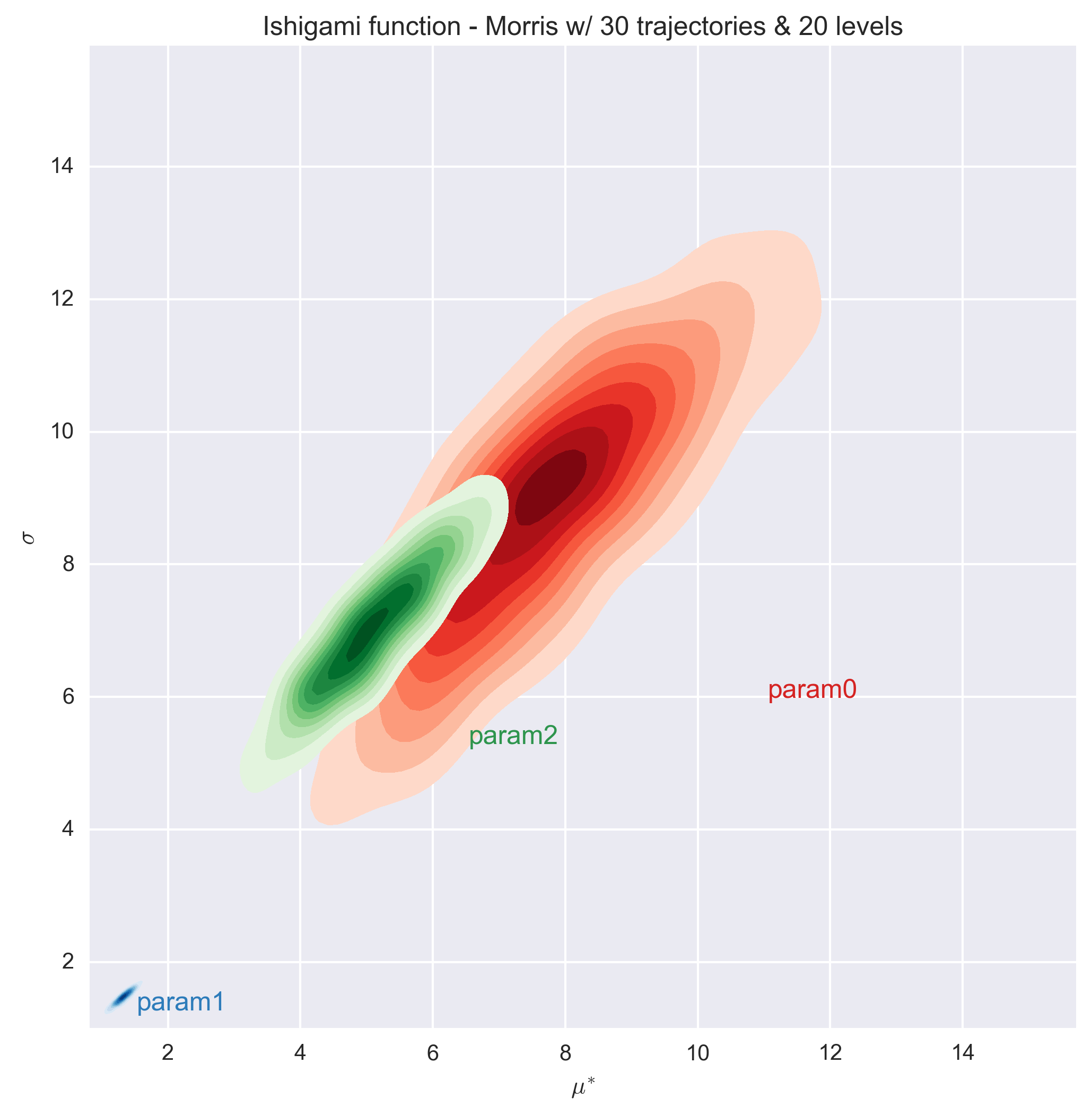
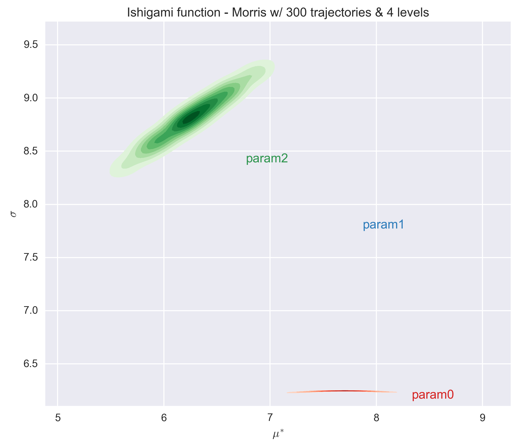
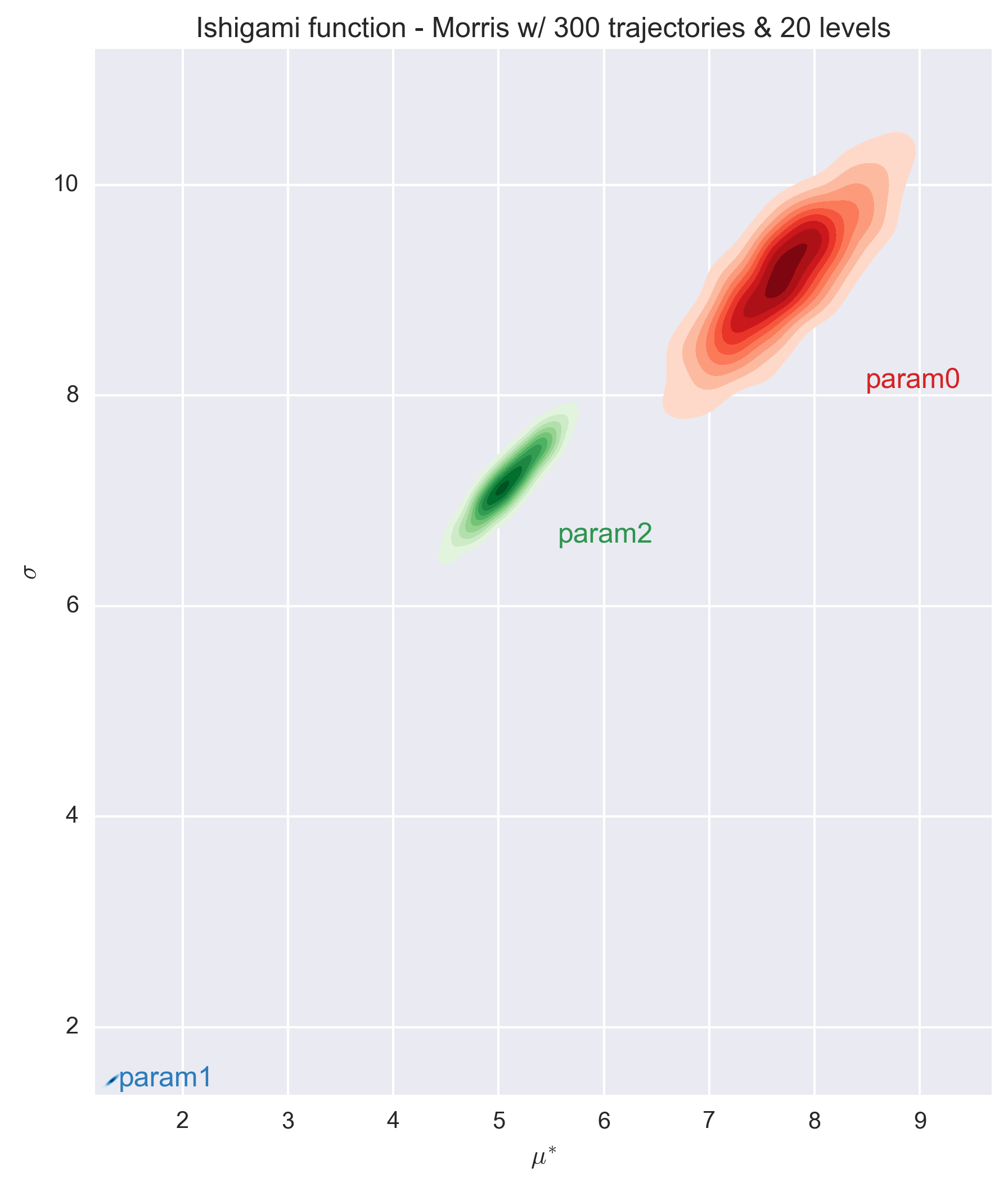
Countrary to the Modified Morris Function, the value of the elementary design with a level p=4 is quite different that the values obtained with the other level values. This remains true for a very large number of trajectories (i.e. 3000). The predictions with a level of 8 or higher are consistent.

We also observe that a number of trajectories equals to 10 times the number of parameter (i.e. 30) is not sufficient to entirely classified the parameters (as the histograms of parameters 0 and 2 overlap). A minimum number of trajectories of about 100 times the number of parameter is necessary for the Ishigami function to separate the parameters.

Radial sampling design

The radial sampling design has been proposed by Campagnolo et al. and is described in more details at Morris Screening Method. Only a number of trajectories, here called blocks to differentiate from the previous design, is required. For testing purposes we investigated, as previously, numbers of blocks (r) equal to 10, 100 and 1000 times the number of parameter (k=3).

Each generated design was used to evaluate the Ishigami function and the associated elementary effects were calculated.

The following figures show the \(\sigma\) vs. \(\mu^*\) plot for the three parameters of the Ishigami function and for the three sets of r values. Countrary to the trajectory design, the radial design uses the Sobol generator, which is deterministic. As such no repetitions were performed to investigate the dispersion of the (\(\sigma\), \(\mu^*\)) values.

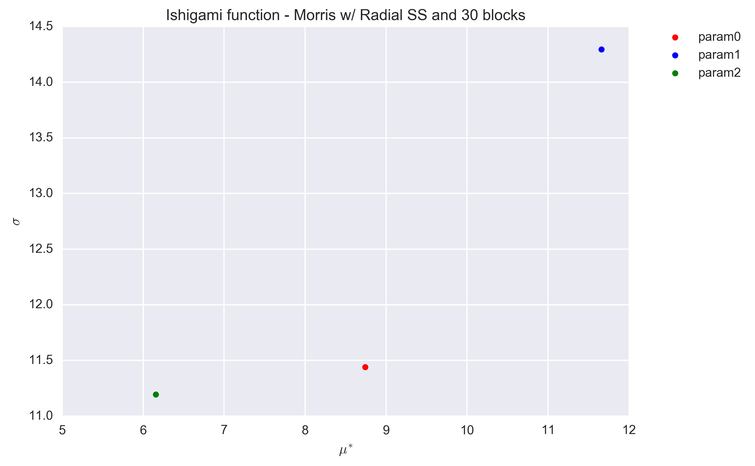
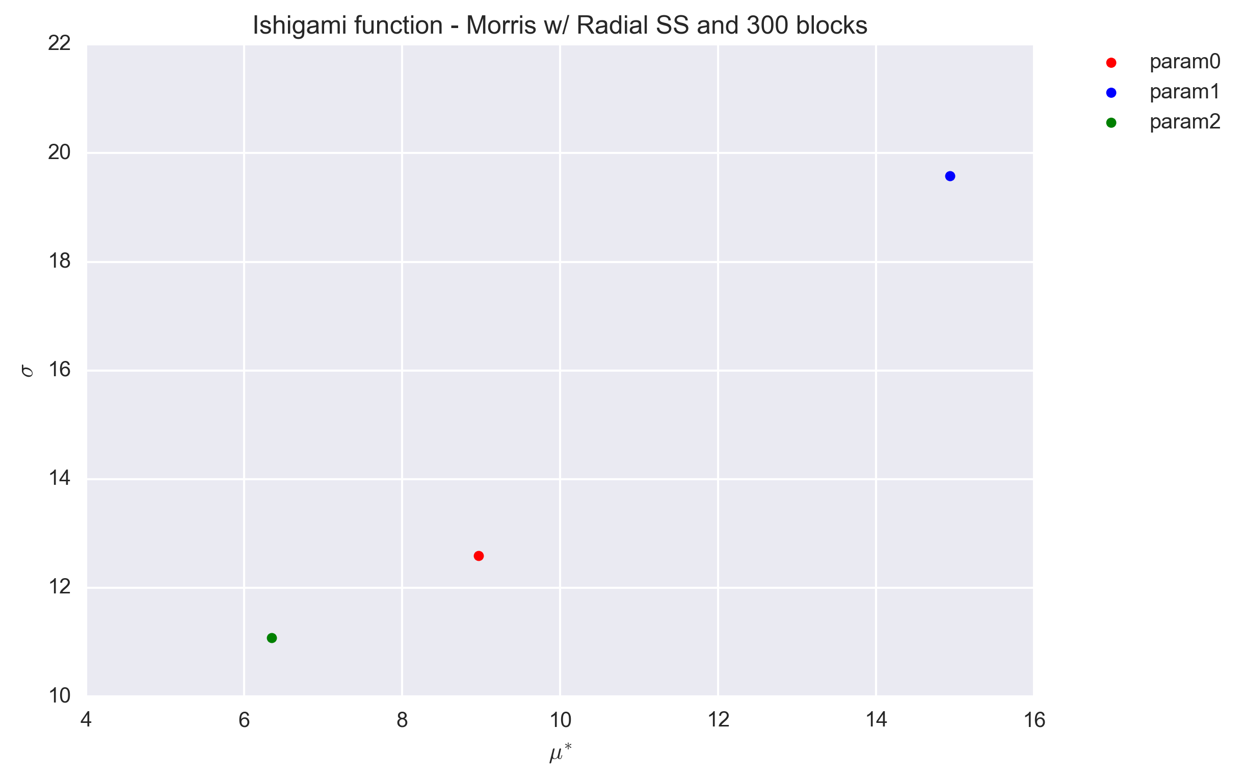
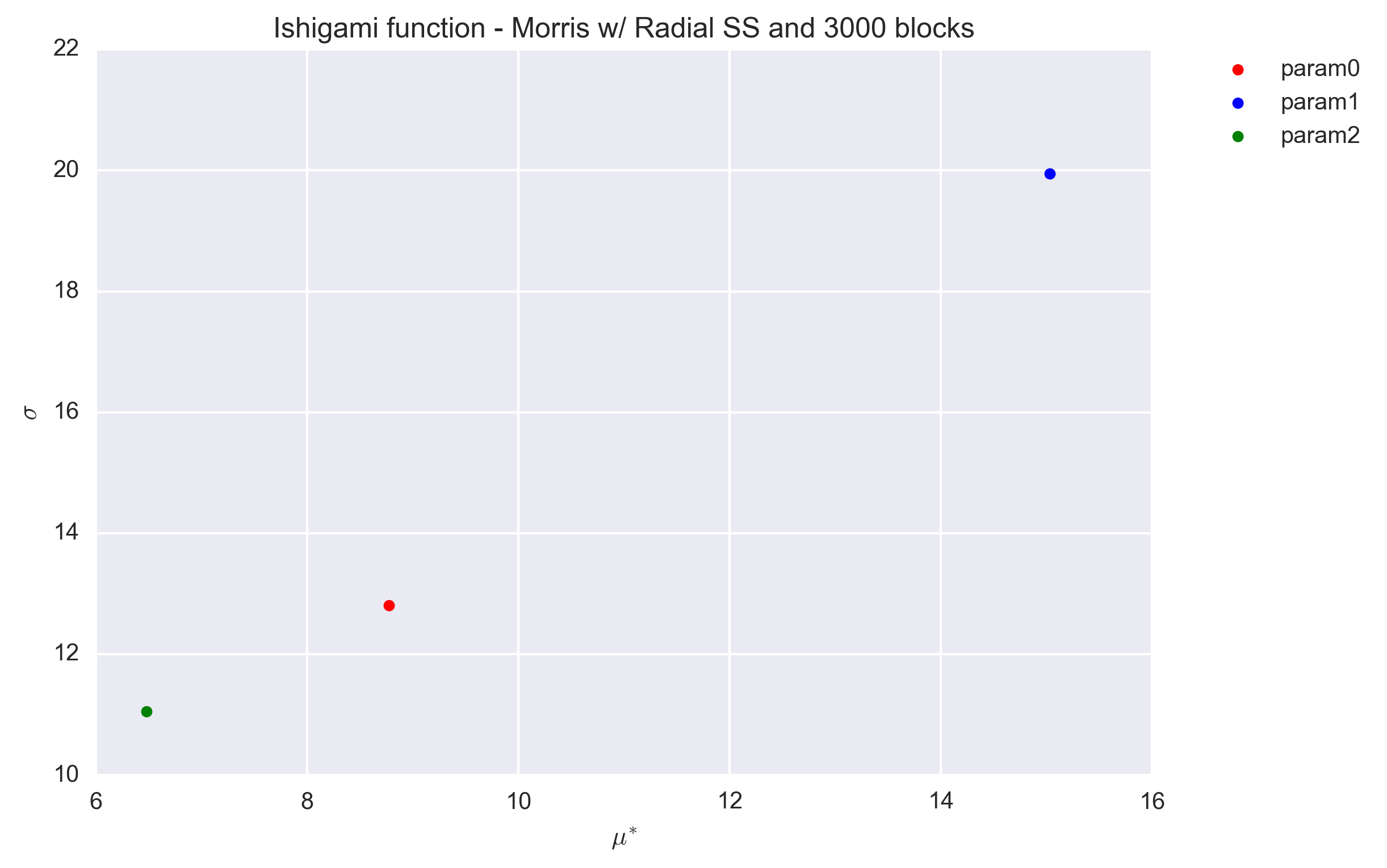
The values are found to be quite stable, even for a block value of r=30. They differ, however, significantly from that obtained with the trajectory design (Section Trajectory sampling design).

The exact value for the elementary effects were not found in litterature. However, the sensitivity indices are \(S_1=0.3138\), \(S_2=0.4424\) and \(S_3=0\) [1]. Because \(\mu^*\) and S quantify the same information, we expect them to be ordered in the same way. Therefore the results obtained with the radial sampling design appear preferable.

Sobol Sensitivity Indices Results

The function was used to test the implementation of the Sobol sensitivity indices. The main-effect (first order) and total-effect (total order) sensitivity indices are both computed. Both the sampling scheme type and the estimator for the sensitivity indices were tested. The tested sampling schemes are simple random sampling (srs), latin-hypercube sampling (lhs) and the sobol sampling (sobol). The tested estimators are janon and saltelli for the main-effect SI and jansen and sobol for the total-effect SI (see Sobol’ Sensitivity Indices).

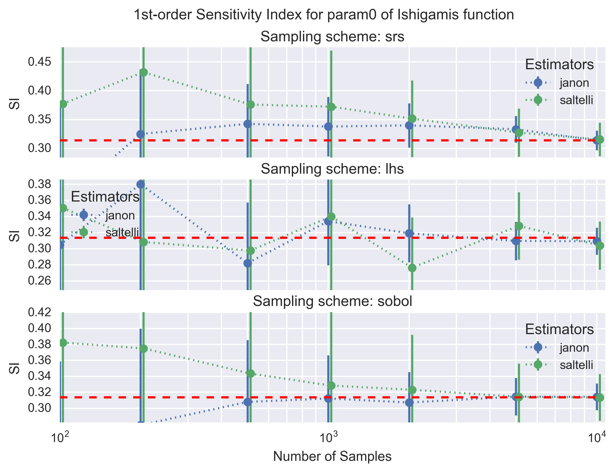
The following figure shows the convergence of the main-effect SI (first order) with the number of samples for the first parameter (param0) of the Ishigami’s function. Each panel shows the janon and saltelli estimators, with their \(1-\sigma\) uncertainties, for a given sampling scheme. The dotted red line is the analytical solution (i.e. the target value).

A similar figure is shown below for the total-effect SI (tot-order) for the jansen and sobol estimators.

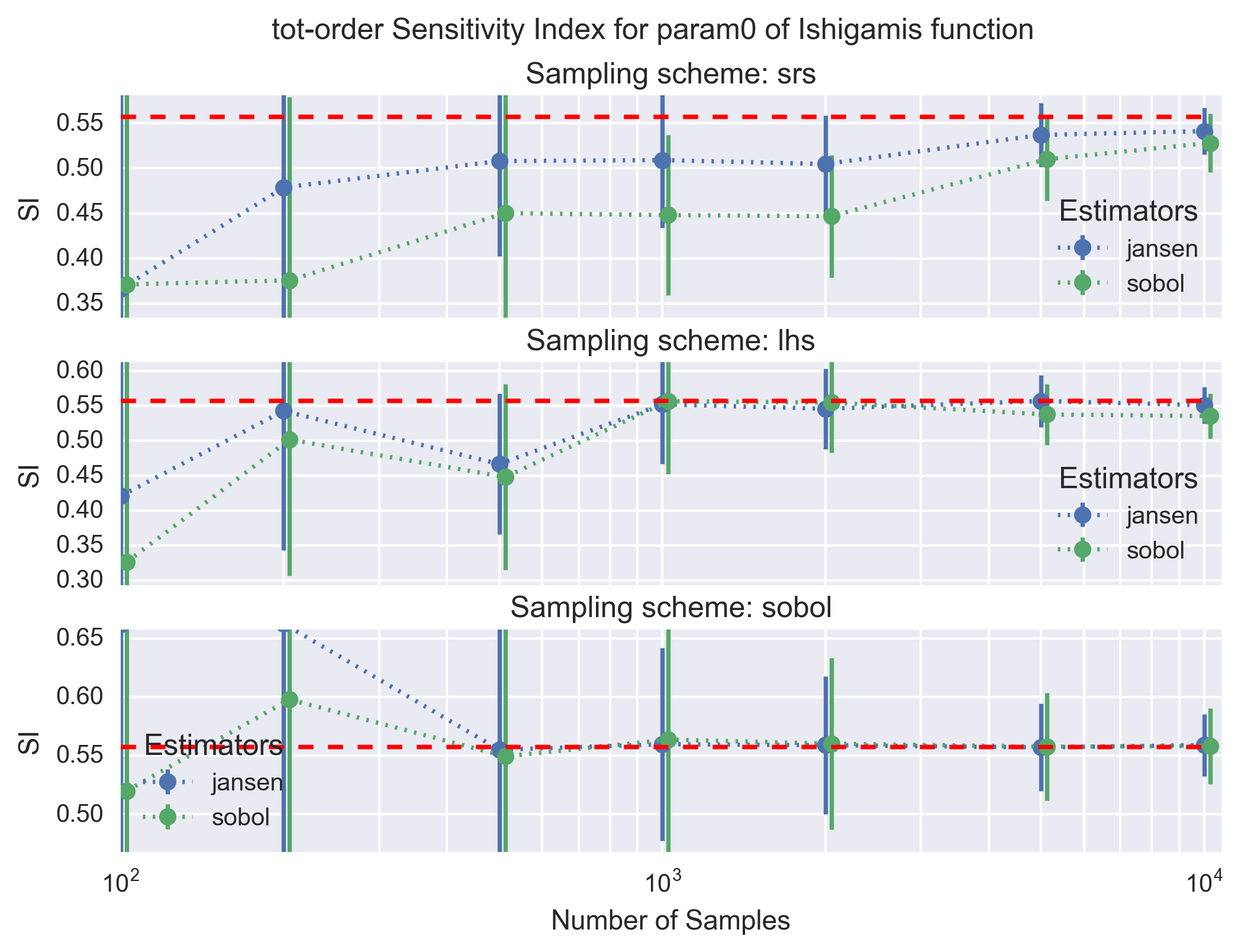
All estimators for the main- and total-effect SI converge to the analytical solution with a sufficient number of samples (i.e. \(10^4\) in the worst case). As expected the sobol and lhs sampling schemes for the design matrix are clearly superior to the simple random scheme (srs) as the calculated main- and total-effect SI converge faster and with a lower uncertainies; the sobol sampling scheme appears to be only slightly better than lhs. Finally, comparing the estimators the janon and jansen estimators show slightly better properties than the saltelli and sobol estimators. These conclusions remain the same for all input parameter of the Ishigami’s function.

From a practical point of view, we advise to use the sobol or lhs sampling scheme with at least 1000 points. The estimator does not play a significant role.

References

[1]	(1, 2) T. Homma and A. Saltelli, “Importance measures in global sensitivity analysis of nonlinear models,” Reliability Engineering and System Safety, vol. 52, pp. 1-17, 1996.

[2]	A. Saltelli et al., “Sensitivity Analysis in Practice,” John Wiley & Sons: West Sussex, 2004, pp. 196