Sobol-\(G^*\) Function

Sobol-\(G^*\) is a modified version of Sobol-G function proposed in [1] initially to avoid excluding singular value at \(\mathbf{x}=\{0.5\}\). The function reads,

\[\begin{split}& G^* (\mathbf{x}, \mathbf{a}, \boldsymbol{\alpha}, \boldsymbol{\delta}) = \prod_{d=1}^D g_i^* \\ & g_d^* = \frac{(1 + \alpha_d) \cdot |2 (x_d + \delta_d - I[x_d + \delta_d]) - 1|^\alpha_d + a_d}{1 + a_d}\end{split}\]

where \(\mathbf{x} \in [0,1]^D\); \(a_d \in \mathbb{R}^+\) determines the first-order importance of parameter-\(d\); \(\delta \in [0,1]^D\) is the shift parameter; \(\boldsymbol{\alpha} \in \mathbb{R}^{D+}\) is the curvature parameter; and \(I[\circ]\) is the integer part of the number.

The parameters \(\mathbf{a}\) and \(\mathbf{\alpha}\) can be adjusted. The particular test function used in this module is \(G_2^*\) (see pp. 265 in [1]) where

\[\begin{split}& \alpha_d = 1; \, d = 1, 2, \cdots, 10 \\ & a_d = (0, 0.1, 0.2, 0.3, 0.4, 0.8, 1, 2, 3, 4) \\ & \delta_d \sim \mathcal{U}[0,1]; \, d = 1, 2, \cdots, 10\end{split}\]

Analytical Solution

The analytical formulas for the variance terms of the Sobol-\(G^*\) function for \(\mathbf{X}_d \sim \mathcal{U}[0,1]; \, d = 1, 2, \cdots, 10\) are the following

Marginal Variance

\[\mathbb{V}[G_2^*] = \left[\prod_{d=1}^D (1 + V_d)\right] - 1\]

where \(V_d\) is the top marginal variance given below,

Top Marginal Variance

\[V_d = \mathbb{V}_{d} [\mathbb{E}_{\sim d} [G_2^*| X_d]] = \frac{\alpha_d^2}{(1 + 2 \alpha_d)(1 + a_d)^2}\]

Bottom Marginal Variance

\[VT_d = \mathbb{E}_{\sim d} [\mathbb{V}_{d} [G_2^* | \mathbf{X}_{\sim d}]] = V_d \prod_{e \neq d} (1 + V_e)\]

The analytical main- and total-effect sensitivity indices can be computed using their respective definition in relation to the variance terms given above.

Sobol Sensitivity Indices Results

The function was used to test the implementation of the Sobol sensitivity indices. The main-effect (first order) and total-effect (total order) sensitivity indices are both computed. Both the sampling scheme type and the estimator for the sensitivity indices were tested. The tested sampling schemes are simple random sampling (srs), latin-hypercube sampling (lhs) and the sobol sampling (sobol). The tested estimators are janon and saltelli for the main-effect SI and jansen and sobol for the total-effect SI (see Sobol’ Sensitivity Indices).

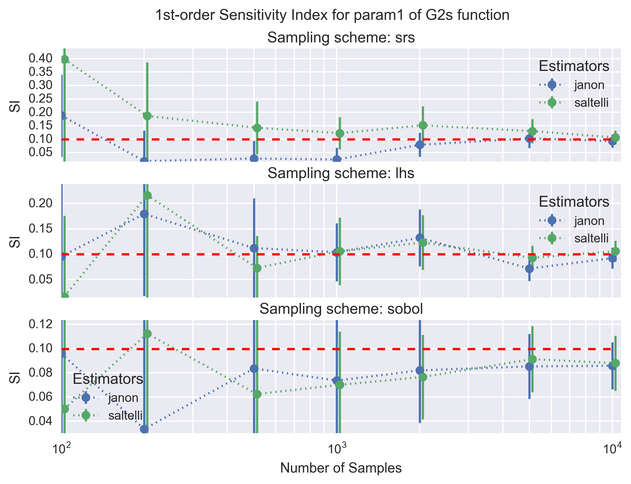
The following figure shows the convergence of the main-effect SI (first order) with the number of samples for the second parameter (param1) of the \(G_2\) function. Each panel shows the janon and saltelli estimators, with their \(1-\sigma\) uncertainties, for a given sampling scheme. The dotted red line is the analytical solution (i.e. the target value).

A similar figure is shown below for the total-effect SI (tot-order) for the jansen and sobol estimators.

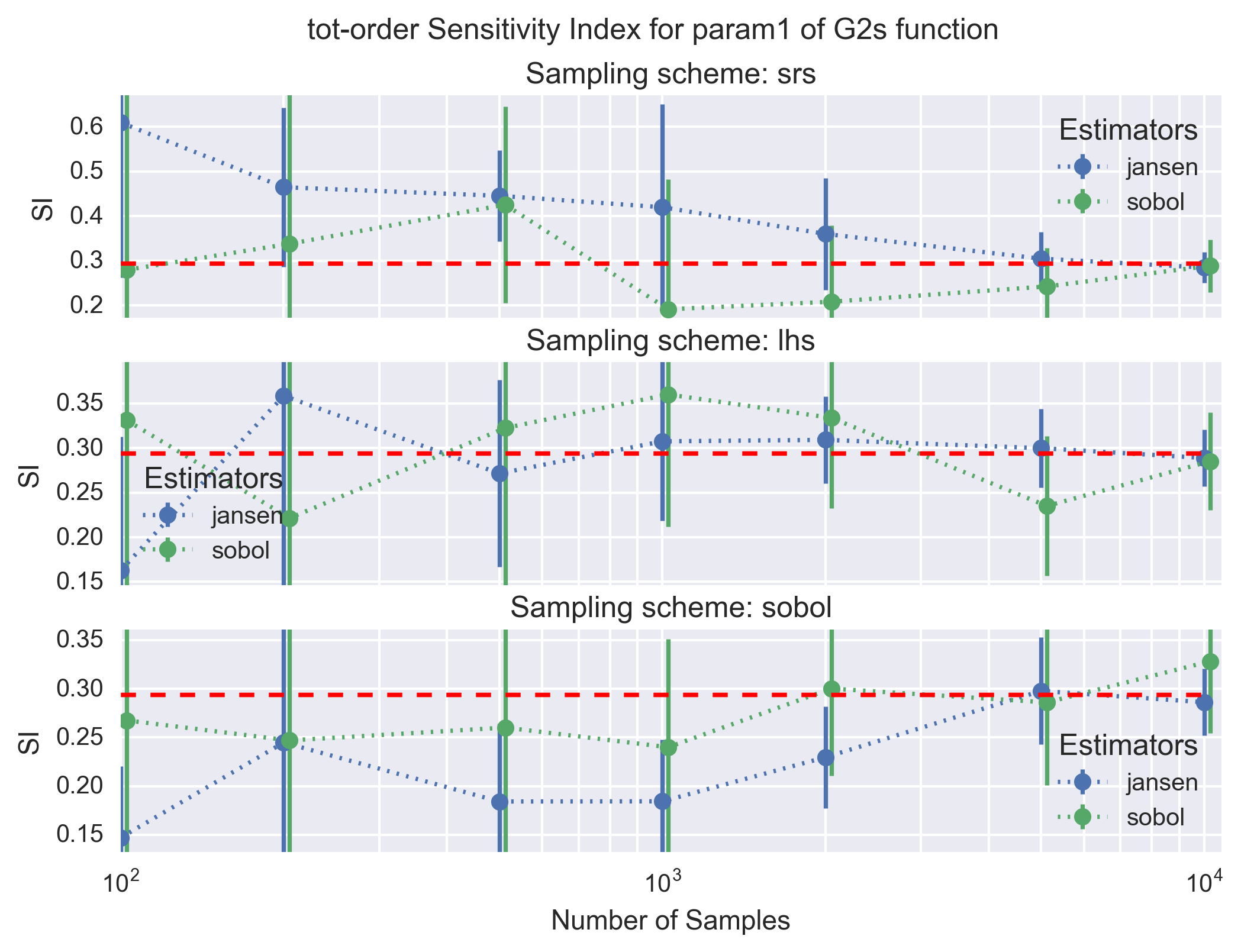
All estimators for the main- and total-effect SI converge to the analytical solution with a sufficient number of samples (i.e. \(10^4\) in the worst case). As expected the sobol and lhs sampling schemes for the design matrix are clearly superior to the simple random scheme (srs) as the calculated main- and total-effect SI converge faster and with a lower uncertainies; the sobol sampling scheme appears to be slightly better than lhs. Finally, comparing the estimators the janon and jansen estimators show slightly better properties than the saltelli and sobol estimators. The better properties of the estimators and sampling schemes illustrated for param1 can vary slightly from parameter to parameter. The convergence of the calculation, however, remains. This confirms the good implementation of the SI calculation routines.

References

[1]	(1, 2) A. Saltelli et al., “Variance based sensitivity analysis of model output. Design and estimator for the total sensitivity index,” Computer Physics Communication, vol. 181, no. 2, pp. 259 - 270, 2010.